Chapter 4 Example II - Lambs Weight

The second example corresponds to identifying anomalous lambs, that may require farmers attention, based on daily weight estimates of individual lambs in a herd. Our goal is to identify anomalous lambs and provide visual tools to examine and understand the anomalies.

The dataset contains data of 80 daily weight estimates for 39 lambs. Data was collected from a novel system (developed by the Volcani PLF lab) which contains electronic scales and drinking behavior sensor, designed for automatic small-ruminant monitoring. The water source is an attraction point, that voluntarily attracts the animals to the scale several times per day.

Loading the necessary packages:

library(MultiNav)
library(corrplot)
library(RColorBrewer)

4.1 Initial Exploration

First we will load and examine the LambsWeight dataset with a basic heat map. We can see that during the 80 days, the lambs gain weight rapidly.

data<-LambsWeight

cols <- rev(colorRampPalette(brewer.pal(6, "Blues"))(100))
lattice::levelplot(data, 
                   col.regions = cols[length(cols):1], 
                   scales=list(y=(list(cex=1)), tck = c(1,0), x=list(cex=1, rot=90)),
                   ylab="Lamb ID",
                   xlab="Days")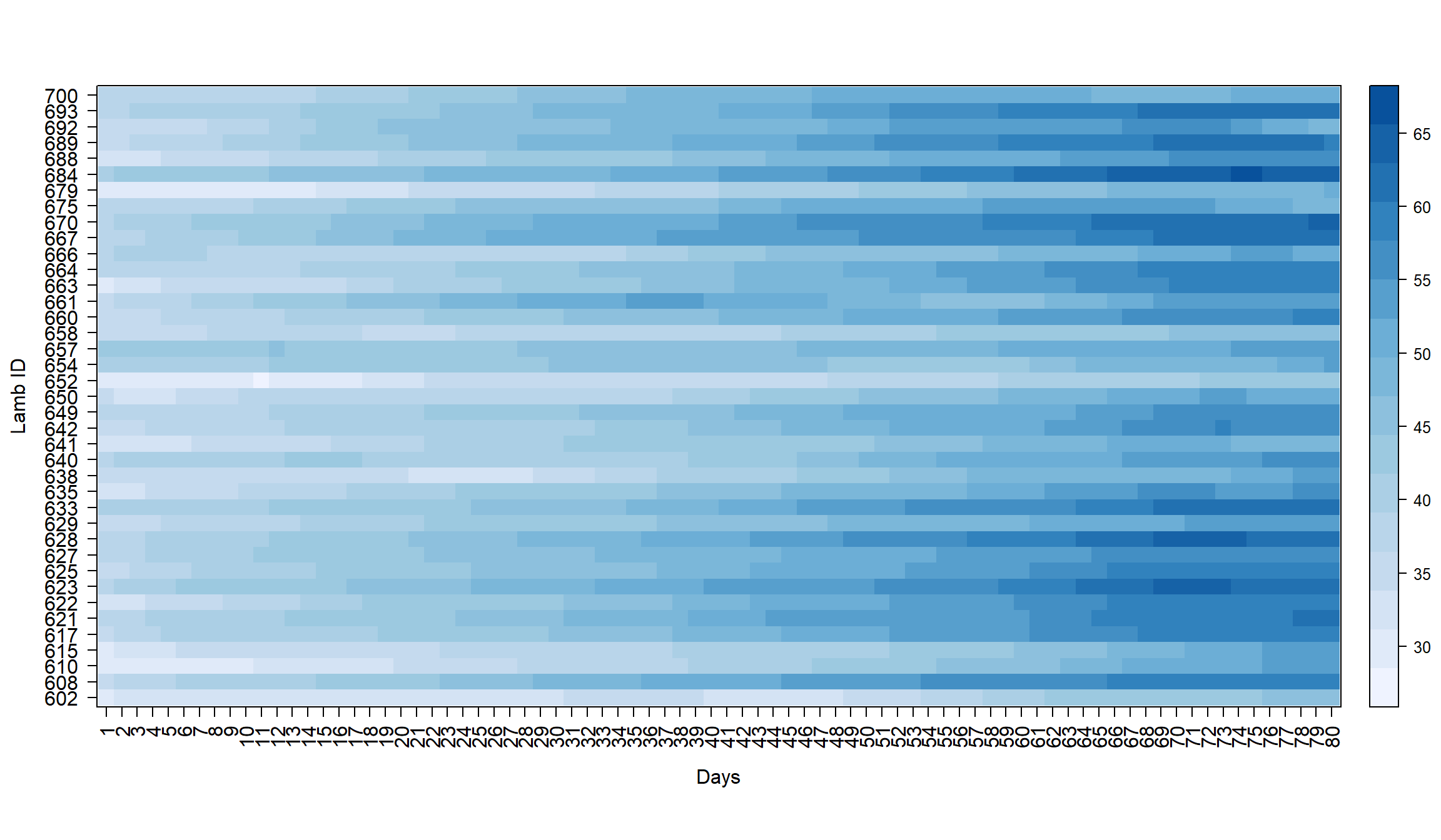 

Then we explore further the data for the whole period of 80 days with MultiNav’s “scores” display using the default univariate scores. Each point in the scatter plot, represents a lamb.

MultiNav(data,type = "scores", xlbl="date id", ylbl="Kg")  

From the functional boxplot background, we see a general growth trend (weight gain). Because we prefer data that is statistically “stable”, we will transform the data and examine the growth-ratio. The anomaly scores that will be calculated in the next sections will be based on the growth-ratio (based on daily weight gaps).

# calculate weight gaps
data_diff<-apply(data, 2, diff)
# calculate the growth-ratio
data_diff_per<-100*data_diff/data[1:dim(data)[1]-1,]
# Call the "scores" display
MultiNav(data_diff_per,type = "scores", xlbl="date id", ylbl="%")

From the functional boxplot background of the growth-ratio we can see that the growth-ratio is slightly decreasing in the first days, stable for the majority of the days, then decreasing again during the last days.

From both of the exploration displays, we can see that during the whole period, there are no extreme outliers (lambs) manifested in the univariate scores.

4.2 Examine Multivariate Outliers

Next we proceed from exploring the whole data with univariate summary statistics, to search for multivariate outliers in a shorter time-window. For each identified anomalous lamb, we would like to understand the nature of the anomaly and review historical anomaly scores.

4.2.1 Sliding Window of “T2_Variations” Scores

As seen in Example I, MultiNav provides set of default multivariate scores. We will start to examine the data with the variations set of Hotelling’s classical \(T^2\) statistic. In order to investigate the nature of each anomaly, we call the “scores” display with the parameter show_diff = TRUE. An additional functional box plot of the differenced data is added, which may provide needed insights regarding the nature of the anomaly.

In this example, the parameter window=3was added, so the input data will be analyzed in a 3 days sliding window and historical scores per lamb are calculated.

Two outlier lambs are identified with the “T2_Variations” scores set for the last sliding window of 3 days. For each identified anomalous lamb, we would like to understand the nature of the anomaly.

The anomaly in lamb 692 is easy to understand as it is manifested in each one of the days (visually seen in the left functional box plot, while lamb 692 is in focus). But for lamb 628, the anomaly is not manifested in any specific day. To understand the nature of the anomaly, we will look at the functional boxplot of differenced data. We see that there is a rapid change in the differenced data which is not typical compared to the difference of the other lambs in the herd (which is relatively constant).

MultiNav(data_diff_per, type = "scores", scores = "T2_Variations",
         window=3, show_diff = TRUE, xlbl="date id")

4.2.2 Sliding Window of “mv” Scores

Next we will calculate anomaly scores for each lamb, using the “mv” default scores set, this time the window parameter is set to 7 (days). Two scores are calculated: 1) T2_MCD75 which seems to work well, identifying 2 anomalies and giving them significantly higher scores then the rest. 2) EigenvectorCentrality method, which does not separate anomalies well for this dataset.

MultiNav(data_diff_per,type = "scores", 
         scores = "mv", window=7, show_diff = TRUE)