Chapter 3 Example I - Dendrometer Sensors
The first example corresponds to the task of identifying malfunctioning dendrometer sensors with unsupervised anomaly detection methods. Dendrometers are measurement devices that continuously monitor size variation in plant organs like stems, branches and fruits. Data from dendrometers can be used for monitoring plants’ daily water status, and make automated irrigation decisions. A major challenge is to identify malfunctioning sensors and filter them out before making irrigation decisions.
Loading the necessary packages:
library(MultiNav)
library(RColorBrewer)
library(data.table)
3.1 Exploratory Data Anaylsis with Univariate Scores
The dendrometer dataset includes data of 100 sensors with 120 hourly readings (5 days). We start by loading the ‘DendrometerSensors’ dataset and performing initial exploration to get a feel of how the data looks like and to check if there are any sensors that have obvious anomalies.
The exploration starts with a simple heatmap. It provides a quick view of the data. The plant organs typically shrink during the day and expand during the night, a pattern that is captured by the dendrometer sensors. The daily growth cycles can be seen clearly in the heatmap. Negative values (red) show the daily shrinkage and positive values (blue) show the night expansion. Visually examining the heatmap, some anomalies can be easily detected, those are the ones that show positive numbers during the day (blue) compared to the majority of the sensors that show negative values (red) during the day.
# Load dataset
data <- DendrometerSensors

# create color palette
cols <- rev(colorRampPalette(c("red", "white", "blue"))(100))

# plot
lattice::levelplot(as.matrix(data),
                   col.regions = cols[length(cols):1],
                   ylab="Dendrometer Id",xlab="Hours") # heatmap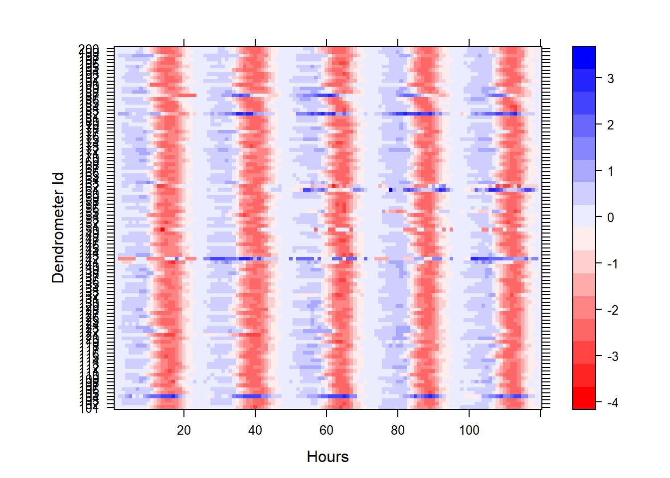
To identify the anomalous sensors and find more subtle anomalies than the ones visible in the heatmap, we will use MultiNav. We start with a battery of univariate, sensor-wise, summary statistics. The selected default univariate summary statistics (per sensor) are the 0.25, 0.5, 0.75 quantiles, and MAD.
Hovering over a sensor in the scatter plots will automatically highlight the sensor in all plots. It will also show the sensor’s raw measurements on a functional box-plot. With this display, we can visually identify several anomalous sensors (104, 142, 161, 182) and investigate the nature of the anomaly, with the functional box-plot.
# Explore data with default set of univariate scores
MultiNav(data, type = "scores", xlbl="Date id")
3.2 Evaluate Multivariate Scoring Methods
The following scoring methods, collectively called “multivariate”, first estimate the correlations within the data (all the data as a single window) and then compute an anomaly score per each sensor. One may think of multivariate scores, as “second order” scores, because they are based on estimate of the correlation between periods.
We propose various methods for computing correlations, and scores. Readers familiar with the multivariate testing literature, will recognize that our various multivariate scores are mostly variations on Hotelling’s classic \(T^2\) statistic. The appropriate method depends on the size of the window, the number of sensors, and the empirical correlations in the data. For this reason, we do not recommend a-priori a single method, but rather, supply the user various such scoring rules.
First, we will examine anomaly scores from a 72 hours window. As pre-processing step, before calculating the anomalies, it is required to remove from the dataset all hours where the standard deviation equals 0. We will do so with MultiNav utility function extract_sd0.
mat<-data[49:120,]      # subset last 72 hours
mat<-extract_sd0(mat)   # Remove rows and column with 0 standard deviation
## 6 rows with 0 standard deviation were omitted.‘MultiNav’ provides two default multivariate anomaly scores sets. The first set contains variations of Hotelling’s classic \(T^2\), calculated using various robust estimators for multivariate location and covariance:
T2_MCD50 - (minimum covariance determinant) estimator. The MCD method looks for the h observations (out of n) whose classical covariance matrix has the lowest possible determinant. In this variation h =0.5*n.
T2_MCD75 - Another variation based on MCD estimator, same as T2_MCD50 with h=0.75*n.
T2_CrouxOllerer - Adaptive method designed to be both robust, and adaptive to high-dimension.
T2_SrivastavaDu - The method is based on assumption of variable independence, useful specifically in super high dimension situations.
set.seed(1236)
MultiNav(mat,type = "scores", scores = "T2_Variations", xlbl="Date id")
Using the “scores” display we can review the sensors that received high score in one of the methods and compare with the scores that the sensor received from the other methods. This way we can learn more about the performance of each method:
T2_CrouxOllerer score had great potential: being designed to be both robust, and adaptive to high-dimension. Alas, in our specific example, it is a poor performer. We suspect this is due to the nature of our data which mostly exhibits very high correlations (above 0.8). Our tests show that the T2_co score performs well in datasets with lower correlation levels.
T2_MCD50 and T2_MCD75 seem to bring similar results, but there are some differences. For instance sensor 142 receives anomalous score only in T2_MCD50 method. In general if there are many outliers in the data set, we may trust more the T2_MCD50 scores.
T2_SrivastavaDu method seems to identify well the anomalies but in general provides lower scores and does not seem to separate the anomalies as cleanly as the robust MCD methods.
Important note: notice how the multivariate scores identified all the anomalies identified by the univariate scores, but also identified several additional sensors (ids 150, 155 and 162).
The second default scores set aims to provide a good default that will be suitable for datasets with various characteristics. However finding a multivariate anomaly default methods is not trivial, our selected methods may work well for some datasets that have certain characteristics but not so well for datasets with other characteristics. The set contains two scoring methods: the T2_MCD75 score (mentioned above) and EigenCent score calculated based on eigenvector centrality, a known network centrality measure.
set.seed(1236)
MultiNav(mat,type = "scores", scores = "mv", xlbl="Date id")3.3 Custom Scores
MultiNav also provides an option for visualizing pre-calculated scores with custom anomaly detection methods. Anomaly scores per sensor can be calculated and then stored in a data.table, data.frame or matrix format. MultiNav() function can receive the custom scores using the scores= argument (limited to four different scores). Here we demonstrate how to create the anomaly scores dataset, creating scores with serval multivariate scoring methods available in MultiNav package.
set.seed(123)
# Calculating multivariate anomaly scores per sensor
T2.score <- T2(t(mat))
T2_mcd75.score <- T2_mcd75(t(mat))
T2_co.score <- round(T2_CrouxOllerer(t(mat)),5)
EigenCent.score<-EigenCentrality(mat)

# Combining the scores into a data.table
Calculated.Scores <- as.data.table(cbind(
  id=as.numeric(colnames(mat)),
  T2=T2.score,
  T2_mcd75=T2_mcd75.score,
  T2_co=T2_co.score,
  EigenCent=EigenCent.score))

# Inspect customized scores dataset
head(Calculated.Scores)
## id T2 T2_mcd75 T2_co EigenCent
## 1: 101 78.99432 62.44049 -2.439843e+15 0.1902445
## 2: 102 26.22013 32.21705 2.412073e+14 0.1702190
## 3: 103 38.72318 44.99511 5.380948e+13 0.1696414
## 4: 104 809.36801 68.67515 -1.457978e+17 1.0000000
## 5: 105 41.91827 52.80158 6.445957e+14 0.1734260
## 6: 106 22.80840 53.90484 -1.718369e+14 0.1727057MultiNav(mat, type = "scores",
scores = Calculated.Scores, xlbl="Date id") MultiNav default scores set are provided as a potential good starting point. Analyst working on a dataset is encouraged to find the multivariate anomaly scores which are most suitable for the specific dataset being analyzed. Then use MultiNav’s visualization tools, by passing the calculated scores as inputs.
3.4 Review Outliers
After examining several anomaly methods and selecting good scoring rules suitable for a specific dataset, typically the next step will be to run the anomaly scores on regular basis on new streaming data, investigating the nature of the identified anomalies. For this purpose, we can also use the “scores” display. This time we will provide as input, a longer data stream containing dendrometers data from 120 time periods. Then we will calculate historical scores in window of size 66 periods. We set the parameter window=66 and also set scores="mv" to call for the default multivariate scores: T2_MCD75 and EigenvectorCentrality.
When using the window parameter, instead of a single summary for the whole data, we compute the summary in a sliding window (beware, calculating historical scores in a sliding window maybe performance intensive). Only the scores from the last window are initially displayed. When clicking on a point representing a sensor, the displays updates. The focus moves to the selected sensor and the sensor’s historical scores are displayed (sliding window scores). This functionality enables to review if there was a trend of improvement or deterioration in the sensor’s historical scores. One may return from the single sensor view, to the all-sensor view, by hitting the “Back to scores” button (upper left corner).
data<-extract_sd0(data)   # Removing rows and column with 0 standard deviation

MultiNav(data, type = "scores", window=66, scores="mv", xlbl="Date id")
Note: the previous examples received input of data from only one time window. To study local patterns, we may want to compute summaries from a longer time frame in a sliding window. Moreover, we may want to account for correlations in each window.